Limits at Infinity and Horizontal Asymptotes

Why this matters¶

On the page Limit Laws we met two resistors in parallel, of 3 ohms and $t$ ohms, with the combined resistance

R(t) = \frac{3t}{3 + t}

(1)

ohms, for $t > 0$ , and we found what it approaches as $t$ approaches 6. Now replace the second resistor by larger and larger ones. What happens to the combined resistance? Rounded, in ohms:

$t = 10$ gives $R(10) \approx 2.3077$ ;
$t = 100$ gives $R(100) \approx 2.9126$ ;
$t = 1000$ gives $R(1000) \approx 2.9910$ ;
$t = 1\,000\,000$ gives $R(1\,000\,000) \approx 2.999991$ .

The values creep up towards 3 and never reach it. Indeed, for every $t > 0$ ,

3 - R(t) = \frac{3(3 + t) - 3t}{3 + t} = \frac{9}{3 + t},

(2)

which is positive, and as small as we like when $t$ is large enough: it is less than 0.001 as soon as $t > 8997$ . A huge resistor in parallel lets almost no current through, so the pair behaves almost like the 3-ohm resistor alone.

This is a new kind of limit. The variable $t$ does not approach a number $a$ : it grows without bound. We will write $\lim_{t \to \infty} R(t) = 3$ , and say that the line $y = 3$ is a horizontal asymptote of the graph of $R$ . We also want to describe $x \to -\infty$ , and values that grow without bound themselves, as $x^2$ does when $x$ grows. This page defines all of these precisely, carries the limit laws over to them, and uses the laws to find the limits of every rational function and of some expressions with square roots.

Limits as $x$ grows without bound¶

Informally, $\lim_{x \to \infty} f(x) = L$ means that $f(x)$ is as close to $L$ as we like for all $x$ large enough. The ε–δ game of the definition of the limit changes in one place: the challenger still names a tolerance $\eps > 0$ , but instead of a window $0 < \abs{x - a} < \delta$ around a point $a$ you reply with a threshold $N$ , and you win if every $x > N$ has $f(x)$ within $\eps$ of $L$ . The window is now the ray of all $x > N$ . For values that grow without bound, such as $x^2$ , the challenger names a height $B$ instead, and you win if $f(x) > B$ for every $x > N$ . Values of $f$ at small $x$ play no part; $f$ only has to be defined from some point on.

Definition 1 (Limits at infinity)

Let $f$ be a function and $L$ a real number.

(a) Let $f$ be defined at every point of an interval $(c, \infty)$ , for some real number $c$ . We say that the limit of $f(x)$ as $x$ tends to infinity is $L$ , and write

\lim_{x \to \infty} f(x) = L,

(3)

if for every $\eps > 0$ there is a real number $N$ such that $f$ is defined at every $x > N$ , and

x > N \quad\text{implies}\quad \abs{f(x) - L} < \eps .

(4)

(b) Let $f$ be defined at every point of an interval $(-\infty, c)$ , for some real number $c$ . We say that the limit of $f(x)$ as $x$ tends to minus infinity is $L$ , and write $\lim_{x \to -\infty} f(x) = L$ , if for every $\eps > 0$ there is a real number $N$ such that $f$ is defined at every $x < N$ , and

x < N \quad\text{implies}\quad \abs{f(x) - L} < \eps .

(5)

(c) Let $f$ be as in (a). We write $\lim_{x \to \infty} f(x) = \infty$ if for every real number $B$ there is a real number $N$ such that $f$ is defined at every $x > N$ , and

x > N \quad\text{implies}\quad f(x) > B ;

(6)

and $\lim_{x \to \infty} f(x) = -\infty$ if the same holds with $f(x) < B$ in place of $f(x) > B$ .

(d) Let $f$ be as in (b). We write $\lim_{x \to -\infty} f(x) = \infty$ , respectively $\lim_{x \to -\infty} f(x) = -\infty$ , if for every real number $B$ there is a real number $N$ such that $f$ is defined at every $x < N$ , and $x < N$ implies $f(x) > B$ , respectively $f(x) < B$ .

We also write $f(x) \to L$ as $x \to \infty$ , and so on. These are the limits at infinity.

In words. Parts (a) and (b) are the game of the definition of the limit with the punctured window $0 < \abs{x - a} < \delta$ replaced by the ray $x > N$ , or $x < N$ . Parts (c) and (d) replace the tolerance band around $L$ by a height $B$ that the values must stay above, or below, from the threshold on. Four points to notice:

If a threshold $N$ wins a round, so does every larger one when $x \to \infty$ (every smaller one when $x \to -\infty$ ): if $N' \ge N$ and $x > N'$ , then $x > N$ by transitivity (property 2 of the order rules). So $N$ may be taken as large as we like, and it depends on $\eps$ (or $B$ ), never on $x$ .
Since $f$ is defined on $(c, \infty)$ in (a), every $N \ge c$ meets the requirement that $f$ be defined at every $x > N$ . That requirement only rules out thresholds that are too small, as the window’s domain clause in the definition of the limit only rules out windows that are too wide.
The symbols $\infty$ and $-\infty$ are not real numbers. “ $\lim_{x \to \infty} f(x) = \infty$ ” does not say that a limit exists: it says how the limit fails to exist as a real number, because the values eventually exceed every real number (property 1 of the remark below proves this). This is the convention that the page Infinite Limits and Vertical Asymptotes uses for infinite limits at a point $a$ (the proposition there proves that such a limit is not a real number). When we say that a limit at infinity exists, we mean that it is a real number.
On the page Infinite Limits and Vertical Asymptotes the heights are $M > 0$ ; that is the same condition, since a threshold that wins the height $\max(B, 1)$ also wins $B$ : if $f(x) > \max(B, 1)$ , then $f(x) > B$ , by transitivity. (For $-\infty$ , the heights there are $-M$ with $M > 0$ , and the height $-\max(-B, 1)$ plays the same role.)

Example. $\lim_{x \to \infty} \frac{1}{x} = 0$ , by part (a). The function is defined at every $x > 0$ , so on $(0, \infty)$ . Let $\eps > 0$ and take $N = \frac{1}{\eps}$ , which is positive by property 6 of the order rules. If $x > N$ , then $0 < \frac{1}{\eps} < x$ , and property 6 gives $\frac{1}{x} < \frac{1}{1/\eps} = \eps$ and $\frac{1}{x} > 0$ . So $\abs{\frac{1}{x} - 0} = \frac{1}{x} < \eps$ , by the definition of the absolute value.

Example. $\lim_{x \to \infty} x^2 = \infty$ , by part (c). Let $B$ be a real number and take $N$ to be the larger of 1 and $B$ . If $x > N$ , then $x > 1$ and $x > B$ . Multiplying $x > 1$ by the positive number $x$ keeps the inequality (property 5(a) of the order rules): $x^2 > x$ . So $x^2 > x > B$ , and $x^2 > B$ by transitivity.

Non-example. No real number $L$ is the limit of $x^2$ as $x \to \infty$ . Take $\eps = 1$ . Whatever $N$ is offered, let $x$ be 1 more than the larger of $N$ and $\abs{L} + 1$ . Then $x > N$ , and $x > \abs{L} + 1 \ge 1$ , so as in the example $x^2 > x > \abs{L} + 1$ . Adding $-L$ to both sides (property 3 of the order rules), and using $\abs{L} - L \ge 0$ (property 3 of the absolute value), gives $x^2 - L > \abs{L} - L + 1 \ge 1$ . So $x^2 - L$ is positive, and $\abs{x^2 - L} = x^2 - L > 1 = \eps$ : the threshold $N$ loses the round $\eps = 1$ .

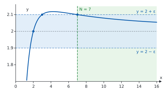
The figure shows one round of the game of part (a).

The graph of y equals (2x squared plus x) over (x squared plus 1) for x from about 1.25 to 16, shown for heights between 1.7 and 2.15 only. A horizontal band runs between the dashed lines y = 1.9 and y = 2.1, with the dotted line y = 2 in its middle. The graph rises steeply, crosses y = 2 at x = 2, leaves the band through its upper edge at x = 3, peaks just above it near x = 4, comes back to the upper edge at x = 7 and then stays inside the band, slowly approaching y = 2 from above. A dashed vertical line marks x = 7, labelled N = 7, and the region to its right is shaded. — Figure 1:The graph of $f(x) = \frac{2x^2 + x}{x^2 + 1}$ , with the band $1.9 < y < 2.1$ of half-width $\eps = 0.1$ around $y = 2$ ; the vertical axis shows only the heights from 1.7 to 2.15. The graph crosses the line $y = 2$ at $x = 2$ , leaves the band at $x = 3$ and returns to it at $x = 7$ . To the right of the threshold $N = 7$ (shaded) it stays inside the band.

For this $\eps$ , the threshold $N = 7$ wins the round, and no smaller threshold does (Exercise 5 proves both). A smaller $\eps$ needs a larger $N$ . The graph meets the line $y = 2$ and leaves the band before it settles: the definition does not care what happens before the threshold.

Before we use the definition, three facts that make it easier to use. The first says that we may speak of the limit at infinity.

Remark 1 (Three facts about limits at infinity)

Uniqueness. A function has at most one limit as $x \to \infty$ , counting $\infty$ and $-\infty$ : if $\lim_{x \to \infty} f(x) = L$ and $\lim_{x \to \infty} f(x) = M$ , where each of $L$ and $M$ is a real number, $\infty$ or $-\infty$ , then $L = M$ . The same holds as $x \to -\infty$ .
Only the tail matters. Let $f$ and $g$ be defined at every point of $(c, \infty)$ , with $f(x) = g(x)$ at every $x > c$ . Then, for $L$ a real number, $\infty$ or $-\infty$ , $\lim_{x \to \infty} f(x) = L$ if and only if $\lim_{x \to \infty} g(x) = L$ . The same holds as $x \to -\infty$ , for $f$ and $g$ defined on $(-\infty, c)$ with $f(x) = g(x)$ at every $x < c$ .
Reflection. Let $f$ be defined at every point of $(-\infty, c)$ , and let $g(t) = f(-t)$ . Then $g$ is defined at every point of $(-c, \infty)$ , and, for $L$ a real number, $\infty$ or $-\infty$ , $\lim_{x \to -\infty} f(x) = L$ if and only if $\lim_{t \to \infty} g(t) = L$ .

Reason. 1. Suppose $L \ne M$ . In each case below we name a round for each of the two limits; let $N_1$ and $N_2$ be thresholds that win them, and let $x$ be 1 more than the larger of $N_1$ and $N_2$ . Then $x > N_1$ and $x > N_2$ , so $f(x)$ is defined and satisfies both inequalities.

$L$ and $M$ real. Take the round $\eps = \frac12 \abs{L - M}$ for both, which is positive by property 1 of the absolute value. By part (b) of the triangle inequality, applied to the numbers $L$ , $M$ and $f(x)$ in the roles of $x$ , $y$ and $z$ there, by property 2 of the absolute value, and by adding the two strict inequalities $\abs{f(x) - L} < \eps$ and $\abs{f(x) - M} < \eps$ (property 4 of the order rules), $\abs{L - M} \le \abs{f(x) - L} + \abs{f(x) - M} < 2\eps = \abs{L - M}$ , which is impossible.
$L$ real and $M = \infty$ . Take $\eps = 1$ for $L$ and $B = L + 1$ for $M$ . Then $\abs{f(x) - L} < 1$ gives $f(x) < L + 1$ , by part (a) of the proposition on distance inequalities, while $f(x) > L + 1$ : impossible, by trichotomy (property 1 of the order rules). For $M = -\infty$ , take $B = L - 1$ : then $f(x) > L - 1$ and $f(x) < L - 1$ .
$L = \infty$ and $M = -\infty$ . Take $B = 0$ for both: then $f(x) > 0$ and $f(x) < 0$ .

The cases with $L$ and $M$ exchanged are the same. As $x \to -\infty$ , let $x$ be 1 less than the smaller of $N_1$ and $N_2$ .

2. If a threshold $N$ wins a round for $f$ , let $N'$ be the larger of $N$ and $c$ . If $x > N'$ , then $x > N$ and $x > c$ , so $g(x)$ is defined and equals $f(x)$ , which satisfies the round’s inequality. So $N'$ wins the same round for $g$ . Exchanging $f$ and $g$ gives the converse. As $x \to -\infty$ , take the smaller of $N$ and $c$ .

3. Multiplying by the negative number ${-1}$ reverses an inequality (property 5(c) of the order rules), so $t > -c$ exactly when $-t < c$ : then $g(t) = f(-t)$ is defined. If $N$ wins a round for $\lim_{x \to -\infty} f(x)$ , then $-N$ wins the same round for $\lim_{t \to \infty} g(t)$ : if $t > -N$ , then $-t < N$ , so $g(t) = f(-t)$ is defined and satisfies the round’s inequality. Conversely, if $N$ wins a round for $g$ , then $-N$ wins it for $f$ : if $x < -N$ , then $-x > N$ , and $f(x) = f(-(-x)) = g(-x)$ .

Horizontal asymptotes¶

A limit at infinity describes the far ends of a graph. When the limit is a real number $L$ , the graph runs ever closer to the horizontal line $y = L$ .

In words. Far to the right, or far to the left, the graph comes as close to the line $y = L$ as we like and stays that close.

Example. The line $y = 3$ is a horizontal asymptote of the graph of the combined resistance $R$ of Why this matters, which is defined only for $t > 0$ , so only the direction $t \to \infty$ is available (Example 5 proves the limit). The line $y = 2$ is a horizontal asymptote of the graph in Figure 1: as the figure shows, a graph may cross its horizontal asymptote.

Non-example. The graph of $x^2$ has no horizontal asymptote. As $x \to \infty$ its limit is $\infty$ , so by property 1 of the remark it is no real number $L$ . As $x \to -\infty$ the same holds, by property 3 of the remark: $g(t) = (-t)^2 = t^2$ .

By property 1 of the remark, a graph has at most two horizontal asymptotes, one for each direction. Each of the two directions may give the same line, a different one, or none.

Horizontal and vertical asymptotes. The page Infinite Limits and Vertical Asymptotes defines a vertical asymptote $x = a$ : a vertical line near which $f(x)$ tends to $\infty$ or to $-\infty$ as $x$ approaches the number $a$ from at least one side. The roles of $x$ and $y$ are exchanged. At a vertical asymptote, $x$ approaches a number and $f(x)$ grows or falls without bound; at a horizontal asymptote, $x$ grows without bound and $f(x)$ approaches a number. A graph may have many vertical asymptotes, but at most two horizontal ones; and it meets a vertical line $x = a$ at most once, because $f$ has at most one value at $a$ , while it may cross a horizontal asymptote. The graph of $\frac{1}{x}$ has both kinds: the line $y = 0$ , as $x \to \infty$ by the example above, and the line $x = 0$ , since $\lim_{x \to 0^{+}} \frac{1}{x} = \infty$ by part (a) of the proposition on reciprocal powers, with $a = 0$ and $n = 1$ .

Main results¶

The limit laws at infinity¶

The limit laws of Limit Laws hold at infinity too, with the same hypotheses. Part (a) differs: the function $x$ has no real limit as $x \to \infty$ , so the identity law becomes a statement about $\infty$ .

Theorem 1 (Limit laws at infinity)

(a) Constants and the identity. For every real number $c$ , $\lim_{x \to \infty} c = c$ and $\lim_{x \to -\infty} c = c$ . Also $\lim_{x \to \infty} x = \infty$ and $\lim_{x \to -\infty} x = -\infty$ .

Now let $f$ and $g$ be functions, each defined at every point of an interval $(\alpha, \infty)$ , for some real number $\alpha$ , such that $\lim_{x \to \infty} f(x) = L$ and $\lim_{x \to \infty} g(x) = M$ , where $L$ and $M$ are real numbers. Then, all limits being taken as $x \to \infty$ :

(b) Sum and difference. $\lim \bigl(f(x) + g(x)\bigr) = L + M$ and $\lim \bigl(f(x) - g(x)\bigr) = L - M$ .
(c) Product. $\lim f(x)\,g(x) = LM$ . In particular, $\lim c\,f(x) = cL$ for every real number $c$ .
(d) Quotient. If $M \ne 0$ , then $\lim \dfrac{f(x)}{g(x)} = \dfrac{L}{M}$ .
(e) Power. For every integer $n \ge 1$ , $\lim \bigl(f(x)\bigr)^n = L^n$ .
(f) Square root. If $L > 0$ , then $\lim \sqrt{f(x)} = \sqrt{L}$ . If $L = 0$ , and there is a real number $K$ such that $f(x) \ge 0$ for every $x > K$ , then $\lim \sqrt{f(x)} = 0$ .

In each of (b)–(f), the function whose limit is taken is defined at every point of some interval $(\alpha', \infty)$ , so that Definition 1 applies to it. The same statements hold as $x \to -\infty$ , for $f$ and $g$ defined on an interval $(-\infty, \alpha)$ , with “for every $x < K$ ” in (f) and intervals $(-\infty, \alpha')$ in the conclusion.

Proof (Sketch)

The proofs on the page Limit Laws carry over with rays in place of windows, and the larger of two thresholds in place of the smaller of two window widths.

Those proofs use the window $0 < \abs{x - a} < \delta$ in only two ways. They take a window from the definition of the limit for each function involved, one round each; and then they take a window inside all of these, $\delta = \min(\delta_1, \delta_2)$ , or the smallest of three. Every inequality after that is about the numbers $f(x)$ and $g(x)$ at one $x$ in that window. At infinity, Definition 1 gives a threshold for each round instead, and the ray $x > N$ with $N = \max(N_1, N_2)$ lies inside both rays $x > N_1$ and $x > N_2$ : if $x > N$ , then $x > N_1$ and $x > N_2$ , by transitivity, since $N \ge N_1$ and $N \ge N_2$ . So each proof carries over with $N = \max(N_1, N_2)$ in place of $\delta = \min(\delta_1, \delta_2)$ , and with its inequalities unchanged.

(b), the sum, written out. Let $\eps > 0$ . There are thresholds $N_1$ and $N_2$ such that $f$ is defined and $\abs{f(x) - L} < \frac{\eps}{2}$ at every $x > N_1$ , and $g$ is defined and $\abs{g(x) - M} < \frac{\eps}{2}$ at every $x > N_2$ . Let $N = \max(N_1, N_2)$ and $x > N$ . Then $f(x)$ and $g(x)$ are defined, and by part (a) of the triangle inequality, then adding the two strict inequalities (property 4 of the order rules),

\begin{aligned} &\abs{\bigl(f(x) + g(x)\bigr) - (L + M)} \\ &\quad \le \abs{f(x) - L} + \abs{g(x) - M} \\ &\quad < \frac{\eps}{2} + \frac{\eps}{2} = \eps . \end{aligned}

(8)

So $f + g$ is defined at every $x > N$ , and $N$ wins the round $\eps$ .

The other parts. (a): for a constant, every $N$ wins every round, since $\abs{c - c} = 0$ . For the identity and a height $B$ , the threshold $N = B$ wins: $x > N$ says that $x > B$ (and as $x \to -\infty$ , $x < N$ says that $x < B$ ). (c): the tolerance 1 gives a threshold beyond which $\abs{f(x)} < \abs{L} + 1$ , and the two tolerances of the product proof on the Limit Laws page give two more; beyond the largest of the three thresholds, that proof’s inequalities hold word for word. (That proof names its constant $N = \abs{M} + 1$ ; this is not our threshold.) (d): the tolerance $\frac{\abs{M}}{2}$ gives a threshold beyond which $\abs{g(x)} > \frac{\abs{M}}{2}$ , so $g(x) \ne 0$ there, and the rest is as in the quotient proof there. (e) is the product law used repeatedly, as in the sketches for the power and square-root laws. (f): the tolerance $L$ gives a threshold beyond which $f(x) > 0$ when $L > 0$ ; when $L = 0$ , the hypothesis gives $f(x) \ge 0$ beyond $K$ ; the inequalities of those sketches then apply at each such $x$ . As $x \to -\infty$ , the rays are $x < N$ , and the smaller of two thresholds replaces the larger.

What this sketch leaves out: writing each of (c)–(f) out with thresholds, including the bookkeeping of the domain, that each new function is defined at every $x$ beyond the final threshold, so on an interval $(N, \infty)$ ; the induction in (e) and the details of (f) that the Limit Laws page itself only sketches; and the versions for $x \to -\infty$ .

(If $f$ and $g$ are defined on two different intervals $(\alpha_1, \infty)$ and $(\alpha_2, \infty)$ , both are defined on the one whose left end is the larger of $\alpha_1$ and $\alpha_2$ , so one $\alpha$ is no restriction.)

When the laws do not apply. As on the Limit Laws page, the laws need the limits $L$ and $M$ of the parts to be real numbers. If both parts tend to $\infty$ , the laws say nothing about the difference, “ $\infty - \infty$ ”, or the quotient, “ $\frac{\infty}{\infty}$ ”, and such limits can be anything. For every real number $c$ , the functions $x + c$ and $x$ both tend to $\infty$ , yet their difference is the constant $c$ , whose limit is $c$ . The quotients $\frac{2x}{x}$ and $\frac{x^2}{x}$ are both “ $\frac{\infty}{\infty}$ ”; they equal 2 and $x$ at every $x > 0$ , so by property 2 of the remark their limits are 2 and $\infty$ , by part (a) of the theorem. Such forms are a signal to rewrite the function first, as the next proof and the examples do.

Rational functions¶

For a rational function, the leading terms decide everything: far out, $\frac{p(x)}{q(x)}$ behaves like the quotient of the leading terms. We first need that the reciprocal powers $\frac{1}{x^j}$ tend to 0.

Proposition 1 (Rational functions at infinity)

(a) For every integer $j \ge 1$ ,

\lim_{x \to \infty} \frac{1}{x^j} = 0 \quad\text{and}\quad \lim_{x \to -\infty} \frac{1}{x^j} = 0 .

(9)

Now let $p$ be a polynomial of degree $m$ with leading coefficient $a$ , let $q$ be a polynomial of degree $k$ with leading coefficient $b$ , and let $r(x) = \frac{p(x)}{q(x)}$ . There is a real number $c \ge 0$ such that $r$ is defined at every $x > c$ and at every $x < -c$ , and:

(b) if $m < k$ , then $\lim_{x \to \infty} r(x) = 0$ and $\lim_{x \to -\infty} r(x) = 0$ ;

(d) if $m > k$ , then $\lim_{x \to \infty} r(x)$ is $\infty$ if $\frac{a}{b} > 0$ and $-\infty$ if $\frac{a}{b} < 0$ ; and $\lim_{x \to -\infty} r(x)$ is $\infty$ if $(-1)^{m - k} \frac{a}{b} > 0$ and $-\infty$ if $(-1)^{m - k} \frac{a}{b} < 0$ .

Proof

We divide the numerator and the denominator by the highest power of $x$ in the denominator, so that every term except the leading ones becomes a constant times a reciprocal power, which tends to 0 by (a); the limit laws at infinity do the rest. The limits as $x \to -\infty$ follow by reflection. Throughout, $a \ne 0$ and $b \ne 0$ , since they are leading coefficients (Definition 1).

Step 1: a power is at least its base. Let $x \ge 1$ . For each integer $i \ge 1$ , $x^i$ is a product of positive numbers, so it is positive (part (d) of the sign rules), and multiplying $1 \le x$ by the positive number $x^i$ gives $x^i \le x^{i + 1}$ (property 5(b) of the order rules). We claim that, for every integer $j \ge 1$ ,

x \le x^j .

(10)

For $j = 1$ this is $x \le x$ ; if $x \le x^j$ , then $x^j \le x^{j + 1}$ (as above) gives $x \le x^{j + 1}$ by transitivity (property 2), so by induction it holds for every $j \ge 1$ .

Step 2: part (a). The function $\frac{1}{x^j}$ is defined at every $x \ne 0$ , since $x^j \ne 0$ there (part (a) of the sign rules). Let $\eps > 0$ , and let $N$ be the larger of 1 and $\frac{1}{\eps}$ . If $x > N$ , then $x > 1$ and $x > \frac{1}{\eps}$ , and by Step 1,

0 < \frac{1}{\eps} < x \le x^j .

(11)

So $\frac{1}{\eps} < x^j$ by transitivity, and property 6 of the order rules gives $0 < \frac{1}{x^j} < \eps$ . So $\abs{\frac{1}{x^j} - 0} = \frac{1}{x^j} < \eps$ (the definition of the absolute value), and $N$ wins the round $\eps$ . As $x \to -\infty$ : by property 3 of the remark we need $\lim_{t \to \infty} \frac{1}{(-t)^j} = 0$ . Since $(-t)^j = (-1)^j t^j$ , and $\frac{1}{(-1)^j} = (-1)^j$ because $(-1)^j (-1)^j = 1$ , this function is $(-1)^j \cdot \frac{1}{t^j}$ , and the “in particular” of part (c) of the limit laws at infinity gives the limit $(-1)^j \cdot 0 = 0$ .

Step 3: where $r$ is defined. By part (a) of the proposition on the domain, $r$ is defined at every real number except the roots of $q$ , of which there are at most $k$ . Let $c$ be the largest of 0 and the absolute values of these roots ( $c = 0$ if $q$ has none). If $x > c$ or $x < -c$ , then $\abs{x} > c$ , because $\abs{x}$ is at least $x$ and at least $-x$ (property 3 of the absolute value); so $x$ is not a root of $q$ , and $x \ne 0$ since $c \ge 0$ . Hence $r$ is defined at $x$ , and $x^k \ne 0$ .

Step 4: the denominator and the numerator, divided by a power. Write $q(x) = b x^k + b_{k-1} x^{k-1} + \dots + b_1 x + b_0$ , and for $x \ne 0$ let

\begin{aligned} Q(x) &= \frac{q(x)}{x^k} \\ &= b + b_{k-1} \cdot \frac{1}{x} \\ &\qquad + \dots + b_0 \cdot \frac{1}{x^k} . \end{aligned}

(12)

By (a) and the “in particular” of part (c) of the laws, each term $b_i \cdot \frac{1}{x^{k - i}}$ with $i < k$ tends to $b_i \cdot 0 = 0$ as $x \to \infty$ ; the constant $b$ tends to $b$ , by part (a) of the laws; and the sum law, part (b), applied once for each term added, gives $\lim_{x \to \infty} Q(x) = b$ . All these functions are defined on $(0, \infty)$ . In the same way, writing $p(x) = a x^m + a_{m-1} x^{m-1} + \dots + a_0$ , the function $P(x) = \frac{p(x)}{x^k}$ tends to $a$ if $m = k$ . If $m < k$ , every term of $P(x)$ is $a_i \cdot \frac{1}{x^{k - i}}$ with $k - i \ge k - m \ge 1$ , so every term tends to 0, and $\lim_{x \to \infty} P(x) = 0$ .

Step 5: parts (b) and (c) as $x \to \infty$ . Since $b \ne 0$ , the quotient law, part (d) of the laws, gives $\lim_{x \to \infty} \frac{P(x)}{Q(x)} = \frac{0}{b} = 0$ if $m < k$ , and $\frac{a}{b}$ if $m = k$ . At every $x > c$ , Step 3 gives $q(x) \ne 0$ and $x^k \ne 0$ , so $Q(x) \ne 0$ and, multiplying the numerator and the denominator by $x^k$ , $\frac{P(x)}{Q(x)} = \frac{p(x)}{q(x)} = r(x)$ . By property 2 of the remark, $r$ has the same limit as $\frac{P}{Q}$ .

Step 6: part (d) as $x \to \infty$ . Let $m > k$ , and for $x > c$ let

S(x) = \frac{p(x) / x^m}{q(x) / x^k} .

(13)

Step 4 with $m$ in place of $k$ gives $\lim_{x \to \infty} \frac{p(x)}{x^m} = a$ , so the quotient law gives $\lim_{x \to \infty} S(x) = \frac{a}{b}$ (with property 2 of the remark, as $S$ is that quotient at every $x > c$ ), and at every $x > c$ , $x^{m - k} S(x) = \frac{p(x)}{q(x)} = r(x)$ .

Suppose first that $\frac{a}{b} > 0$ , and let $h = \frac12 \cdot \frac{a}{b}$ , which is positive. With the tolerance $h$ , there is a threshold $N_1$ such that $\abs{S(x) - \frac{a}{b}} < h$ at every $x > N_1$ , and then $S(x) > \frac{a}{b} - h = h$ , by part (a) of the proposition on distance inequalities. Let $B$ be a real number, let $N$ be the largest of $N_1$ , $c$ , 1 and $\frac{\abs{B}}{h}$ , and let $x > N$ . Then $r(x)$ is defined (Step 3), $S(x) > h > 0$ , and $x > 1$ , so $x^{m - k} \ge x$ by Step 1, as $m - k \ge 1$ . Multiplying $x^{m - k} \ge x$ by the positive number $S(x)$ , multiplying $S(x) > h$ by the positive number $x$ , and multiplying $x > \frac{\abs{B}}{h}$ by the positive number $h$ (property 5 of the order rules) gives

\begin{aligned} r(x) &= x^{m - k} S(x) \\ &\ge x\,S(x) > x h \\ &> \abs{B} \ge B , \end{aligned}

(14)

where $\abs{B} \ge B$ is property 3 of the absolute value. So $r(x) > B$ by transitivity, and $\lim_{x \to \infty} r(x) = \infty$ .

If $\frac{a}{b} < 0$ , apply this to $-p$ , which has degree $m$ and leading coefficient $-a$ , with $\frac{-a}{b} > 0$ : so $\lim_{x \to \infty} \bigl(-r(x)\bigr) = \infty$ . Given a real number $B$ , a threshold that wins the round $-B$ for $-r$ wins the round $B$ for $r$ with “ $<$ ”: $-r(x) > -B$ gives $r(x) < B$ , multiplying by the negative number ${-1}$ , which reverses the inequality (property 5(c) of the order rules). So $\lim_{x \to \infty} r(x) = -\infty$ .

Step 7: the limits as $x \to -\infty$ . Let $\tilde p(t) = p(-t)$ and $\tilde q(t) = q(-t)$ . Since $(-t)^i = (-1)^i t^i$ , the polynomial $\tilde p$ has the coefficient $(-1)^i a_i$ at $t^i$ ; at $t^m$ this is $(-1)^m a$ , which is not 0 (part (a) of the sign rules), and there are no higher powers. So $\tilde p$ has degree $m$ and leading coefficient $(-1)^m a$ , and likewise $\tilde q$ has degree $k$ and leading coefficient $(-1)^k b$ . The rational function $\tilde r = \frac{\tilde p}{\tilde q}$ has $\tilde r(t) = r(-t)$ , and $r$ is defined at every $x < -c$ (Step 3). By property 3 of the remark, $\lim_{x \to -\infty} r(x)$ is $\lim_{t \to \infty} \tilde r(t)$ , which Steps 5 and 6 give, with $(-1)^m a$ and $(-1)^k b$ in place of $a$ and $b$ . If $m < k$ , it is 0. If $m = k$ , it is $\frac{(-1)^m a}{(-1)^m b} = \frac{a}{b}$ . If $m > k$ , the sign that decides is that of

\frac{(-1)^m a}{(-1)^k b} = (-1)^{m - k} \frac{a}{b},

(15)

because $(-1)^m = (-1)^{m - k} (-1)^k$ .

In words. Compare the degrees. A higher degree in the denominator pulls the quotient to 0; equal degrees give the quotient $\frac{a}{b}$ of the leading coefficients; a higher degree in the numerator sends the quotient to $\infty$ or $-\infty$ , with the sign of $\frac{a x^m}{b x^k} = \frac{a}{b} x^{m - k}$ far out on that side. So the graph of $r$ has the horizontal asymptote $y = 0$ in case (b), $y = \frac{a}{b}$ in case (c), in both directions, and none in case (d).

Example. $\frac{3x^2 - x + 2}{2x^2 + 5}$ has $m = k = 2$ , so its limit in both directions is $\frac{3}{2}$ . Non-example. For $\frac{x^2 + 1}{x}$ , $m = 2 > k = 1$ and $\frac{a}{b} = 1$ : the limit is $\infty$ as $x \to \infty$ , and, since $(-1)^1 \cdot 1 < 0$ , $-\infty$ as $x \to -\infty$ . There is no horizontal asymptote.

Comparing growth¶

Limits at infinity let us say which of two functions grows faster. Informally, $f$ grows faster than $g$ as $x \to \infty$ if $\frac{g(x)}{f(x)} \to 0$ : eventually $g(x)$ is a tiny fraction of $f(x)$ .

Higher powers grow faster. If $m > k \ge 0$ , then $\frac{x^k}{x^m} = \frac{1}{x^{m - k}}$ for $x \ne 0$ , which tends to 0 by part (a) of the proposition. So $x^3$ grows faster than $1000 x^2$ , although $1000 x^2$ is far larger for a long time: at $x = 10$ it is $100\,000$ against 1000, at $x = 1000$ the two are equal, and at $x = 10\,000$ , $x^3$ is ten times larger.
A polynomial grows like its leading term. By part (c) of the proposition, applied to $p(x)$ over its leading term $a x^m$ , $\frac{p(x)}{a x^m} \to 1$ : the other terms become negligible in comparison.
The square root grows, but more slowly than $x$ . $\sqrt{x}$ eventually exceeds every height (Exercise 13), yet $\frac{\sqrt{x}}{x + 1} \to 0$ (Exercise 8).

Worked examples¶

From the definition¶

Example 1 (Prove

\lim_{x \to \infty} \frac{2x}{x + 1} = 2

from the definition)

Goal. Given $\eps > 0$ , find a threshold $N$ such that $x > N$ implies $\abs{\frac{2x}{x + 1} - 2} < \eps$ . The function $f(x) = \frac{2x}{x + 1}$ is defined at every $x \ne -1$ , so on $(-1, \infty)$ , and part (a) of Definition 1 applies.

Scratch work. For $x > -1$ , $x + 1 > 0$ , and
$\begin{aligned} f(x) - 2 &= \frac{2x - 2(x + 1)}{x + 1} \\ &= \frac{-2}{x + 1} . \end{aligned}$
(16)
By property 4 of the absolute value, and since $x + 1 > 0$ , $\abs{f(x) - 2} = \frac{2}{x + 1}$ .
Choose $N$ . We need $\frac{2}{x + 1} < \eps$ . Since $x + 1 > 0$ , multiplying by $\frac{x + 1}{\eps} > 0$ shows this holds exactly when $x + 1 > \frac{2}{\eps}$ , that is, $x > \frac{2}{\eps} - 1$ . So take $N = \frac{2}{\eps} - 1$ . It depends on $\eps$ only, and $N > -1$ , so $f$ is defined at every $x > N$ .
Proof. Let $\eps > 0$ , $N = \frac{2}{\eps} - 1$ and $x > N$ . Adding 1 to both sides, $x + 1 > \frac{2}{\eps} > 0$ . By property 6 of the order rules, $\frac{1}{x + 1} < \frac{\eps}{2}$ , and multiplying by the positive number 2 keeps the inequality:
$\begin{aligned} \abs{f(x) - 2} &= \frac{2}{x + 1} \\ &< 2 \cdot \frac{\eps}{2} = \eps . \end{aligned}$
(17)

\boxed{N = \frac{2}{\eps} - 1}

(18)

No smaller threshold wins: at $x = \frac{2}{\eps} - 1$ itself, $\abs{f(x) - 2} = \eps$ , not less.

Check. For $\eps = 0.1$ : $N = 19$ , and $x = 20$ gives $f(20) = \frac{40}{21} \approx 1.904762$ , which is $\frac{2}{21} \approx 0.095 < 0.1$ from 2. ✓

Rational functions¶

Example 2 (Three rational functions)

Find (i) $\displaystyle \lim_{x \to \infty} \frac{3x^2 - x + 2}{2x^2 + 5}$ , (ii) $\displaystyle \lim_{x \to -\infty} \frac{x + 4}{x^2 + 1}$ and (iii) $\displaystyle \lim_{x \to -\infty} \frac{x^3 - 2x}{4x^2 + 1}$ .

(i) The degrees are $m = k = 2$ , and the leading coefficients $a = 3$ and $b = 2$ . By part (c) of Proposition 1, the limit is $\frac{3}{2}$ . By hand, as in the proof: for $x \ne 0$ , dividing the numerator and the denominator by $x^2$ ,
$\frac{3x^2 - x + 2}{2x^2 + 5} = \frac{3 - \frac{1}{x} + \frac{2}{x^2}}{2 + \frac{5}{x^2}},$
(19)
and by part (a) of the proposition and the laws of Theorem 1, the numerator tends to $3 - 0 + 2 \cdot 0 = 3$ and the denominator to $2 + 5 \cdot 0 = 2 \ne 0$ .
(ii) Here $m = 1 < k = 2$ . By part (b) of the proposition, the limit is 0.
(iii) Here $m = 3 > k = 2$ , $a = 1$ and $b = 4$ , so $\frac{a}{b} = \frac{1}{4}$ . As $x \to -\infty$ , part (d) of the proposition looks at the sign of $(-1)^{3 - 2} \cdot \frac{1}{4} = -\frac{1}{4}$ , which is negative. So the limit is $-\infty$ . Far to the left the function behaves like $\frac{x^3}{4x^2} = \frac{x}{4}$ , which is very negative there.

\boxed{\text{(i) } \frac{3}{2} \qquad \text{(ii) } 0 \qquad \text{(iii) } -\infty}

(20)

The graph of (i) has the horizontal asymptote $y = \frac{3}{2}$ in both directions, that of (ii) the asymptote $y = 0$ , and that of (iii) none.

Check. (i) At $x = 1000$ the function is $\frac{2\,999\,002}{2\,000\,005} \approx 1.499497$ . ✓ (ii) At $x = -1000$ it is about ${-0.000996}$ . ✓ (iii) At $x = -100$ it is about ${-24.99}$ , and at $x = -1000$ about ${-250.00}$ . ✓

Square roots¶

Example 3 (A difference of two large numbers:

\lim_{x \to \infty} \bigl(\sqrt{x^2 + 1} - x\bigr)

)

The laws do not apply directly. $\sqrt{x^2 + 1}$ is defined for every $x$ , since $x^2 + 1 > 0$ . Both $\sqrt{x^2 + 1}$ and $x$ grow without bound, and the difference law needs real limits: this is “ $\infty - \infty$ ”.
Multiply by the conjugate. For every real $x$ , $\abs{x}^2 = x^2 < x^2 + 1$ (property 5 of the absolute value), and both $\abs{x}$ and $\sqrt{x^2 + 1}$ are non-negative, so the order part of the square-root remark gives $\abs{x} < \sqrt{x^2 + 1}$ . With $-x \le \abs{x}$ (property 3 of the absolute value), $\sqrt{x^2 + 1} + x > 0$ . So we may divide by it, at every $x$ . Using $\bigl(\sqrt{y}\bigr)^2 = y$ for $y \ge 0$ ,
$\begin{aligned} &\bigl(\sqrt{x^2 + 1} - x\bigr)\bigl(\sqrt{x^2 + 1} + x\bigr) \\ &\quad = (x^2 + 1) - x^2 = 1 , \end{aligned}$
(21)
and dividing by $\sqrt{x^2 + 1} + x$ ,
$\sqrt{x^2 + 1} - x = \frac{1}{\sqrt{x^2 + 1} + x} .$
(22)
This is an identity at every $x$ , not only near some point.
Take out $x$ under the root. For $x > 0$ , the number $x\sqrt{1 + \frac{1}{x^2}}$ is non-negative, and its square is $x^2 \bigl(1 + \frac{1}{x^2}\bigr) = x^2 + 1$ . By the uniqueness in the square-root remark, it is $\sqrt{x^2 + 1}$ . Dividing the numerator and the denominator by $x > 0$ ,
$\frac{1}{\sqrt{x^2 + 1} + x} = \frac{\frac{1}{x}}{\sqrt{1 + \frac{1}{x^2}} + 1} .$
(23)
The laws. By part (a) of Proposition 1, $\frac{1}{x^2} \to 0$ , so $1 + \frac{1}{x^2} \to 1$ (parts (a) and (b) of Theorem 1). Since $1 > 0$ , part (f) gives $\sqrt{1 + \frac{1}{x^2}} \to \sqrt{1} = 1$ , so the denominator tends to $2 \ne 0$ . The numerator tends to 0, by part (a) of the proposition, and the quotient law, part (d), gives the limit $\frac{0}{2} = 0$ .
Back to the function. The last quotient equals $\sqrt{x^2 + 1} - x$ at every $x > 0$ , so by property 2 of the remark the two have the same limit.

\boxed{\lim_{x \to \infty} \bigl(\sqrt{x^2 + 1} - x\bigr) = 0}

(24)

Check. At $x = 1000$ : $\sqrt{1\,000\,001} - 1000 \approx 0.0005$ , and $\frac{1}{\sqrt{1\,000\,001} + 1000} \approx \frac{1}{2000}$ . ✓

Example 4 (Two different horizontal asymptotes)

Find the horizontal asymptotes of the graph of $f(x) = \dfrac{x}{\sqrt{x^2 + 1}}$ .

Domain. $x^2 + 1 \ge 1 > 0$ for every $x$ , so $\sqrt{x^2 + 1}$ is defined and positive, and $f$ is defined on $\R$ .
Take out $\abs{x}$ under the root. For $x \ne 0$ , the number $\abs{x}\sqrt{1 + \frac{1}{x^2}}$ is non-negative, and its square is $\abs{x}^2 \bigl(1 + \frac{1}{x^2}\bigr) = x^2 + 1$ , by property 5 of the absolute value. By the uniqueness in the square-root remark,
$\sqrt{x^2 + 1} = \abs{x}\sqrt{1 + \frac{1}{x^2}} .$
(25)
It is $\abs{x}$ , not $x$ , that comes out.
As $x \to \infty$ . For $x > 0$ , $\abs{x} = x$ , so $f(x) = \dfrac{1}{\sqrt{1 + 1/x^2}}$ . By part (a) of Proposition 1, $\frac{1}{x^2} \to 0$ , so by parts (a), (b) and (f) of Theorem 1, $\sqrt{1 + \frac{1}{x^2}} \to \sqrt{1} = 1$ , which is not 0, and the quotient law gives the limit $\frac{1}{1} = 1$ . By property 2 of the remark, $\lim_{x \to \infty} f(x) = 1$ .
As $x \to -\infty$ . For $x < 0$ , $\abs{x} = -x$ (the definition of the absolute value), so
$\begin{aligned} f(x) &= \frac{x}{-x\sqrt{1 + 1/x^2}} \\ &= -\frac{1}{\sqrt{1 + 1/x^2}} . \end{aligned}$
(26)
By part (a) of Proposition 1, $\frac{1}{x^2} \to 0$ as $x \to -\infty$ too. The laws as $x \to -\infty$ then work as in step 3: by parts (a), (b) and (f) of Theorem 1, $\sqrt{1 + \frac{1}{x^2}} \to 1$ , which is not 0; the quotient law gives $\frac{1}{\sqrt{1 + 1/x^2}} \to 1$ ; and the “in particular” of part (c), with the factor ${-1}$ , gives the limit -1. The formula holds at every $x < 0$ , so by property 2 of the remark, in its form for $x \to -\infty$ , $\lim_{x \to -\infty} f(x) = -1$ .

\boxed{ \begin{aligned} \lim_{x \to \infty} f(x) &= 1 \\ \lim_{x \to -\infty} f(x) &= -1 \end{aligned} }

(27)

So the graph has two horizontal asymptotes, $y = 1$ on the right and $y = -1$ on the left. This cannot happen for a rational function: by Proposition 1, its two limits, when real, are equal.

Check. $f(1000) \approx 0.9999995$ and $f(-1000) \approx {-0.9999995}$ . The sign is right: $f(x)$ has the sign of $x$ , since the denominator is positive. ✓

An application¶

Example 5 (A very large resistor in parallel)

Find $\lim_{t \to \infty} R(t)$ for the combined resistance $R(t) = \frac{3t}{3 + t}$ ohms, $t > 0$ , of Why this matters, and how large the second resistor must be for $R(t)$ to be within 0.01 ohm of the limit.

The function. $R$ is defined on $(0, \infty)$ , and it agrees there with the rational function $r(t) = \frac{3t}{t + 3}$ , defined at every $t \ne -3$ .
The limit. For $r$ , the degrees are $m = k = 1$ and the leading coefficients $a = 3$ and $b = 1$ , so by part (c) of Proposition 1, $\lim_{t \to \infty} r(t) = 3$ . By property 2 of the remark, with $c = 0$ , $\lim_{t \to \infty} R(t) = 3$ .
How large? For $t > 0$ , $\abs{R(t) - 3} = 3 - R(t) = \frac{9}{3 + t}$ , as in Why this matters. This is less than 0.01 exactly when $3 + t > 900$ (multiply by the positive number $\frac{3 + t}{0.01}$ , or divide by it, which keeps the inequality), that is, when $t > 897$ .

\boxed{\lim_{t \to \infty} R(t) = 3}

(28)

The combined resistance approaches 3 ohms, and it is within 0.01 ohm of 3 ohms exactly when the second resistor has more than 897 ohms: for $\eps = 0.01$ , the threshold $N = 897$ wins. The line $y = 3$ is a horizontal asymptote of the graph of $R$ .

Check. $R(897) = \frac{2691}{900} = 2.99$ , exactly 0.01 below 3, and $R(898) = \frac{2694}{901} \approx 2.990011$ . ✓ Units: ohms times ohms over ohms is ohms. ✓ A parallel combination is smaller than each resistor, and $R(t) < 3$ . ✓

Common mistakes¶

“

\sqrt{x^2} = x

”, also as

x \to -\infty

✗ Wrong: “ $\dfrac{x}{\sqrt{x^2 + 1}} = \dfrac{x}{x\sqrt{1 + 1/x^2}} = \dfrac{1}{\sqrt{1 + 1/x^2}}$ , so the limit as $x \to -\infty$ is 1.”

Why: $\sqrt{x^2} = \abs{x}$ (property 5 of the absolute value), and for $x < 0$ that is $-x$ , not $x$ . A square root is never negative, so taking $x$ out of $\sqrt{x^2 + 1}$ for negative $x$ produces the wrong sign. At $x = -10$ the function is about ${-0.995}$ , nowhere near 1.

✓ Right: $\sqrt{x^2 + 1} = \abs{x}\sqrt{1 + 1/x^2} = -x\sqrt{1 + 1/x^2}$ for $x < 0$ , and the limit as $x \to -\infty$ is ${-1}$ (Example 4). Treat $x \to \infty$ and $x \to -\infty$ separately whenever a square root of $x^2$ appears.

“

\infty - \infty = 0

”

✗ Wrong: “ $\sqrt{x^2 + x}$ and $x$ both tend to $\infty$ , so $\lim_{x \to \infty} \bigl(\sqrt{x^2 + x} - x\bigr) = \infty - \infty = 0$ .”

Why: $\infty$ is not a number, and the difference law needs both limits to be real numbers. “ $\infty - \infty$ ” can hide any value: $(x + c) - x$ has the limit $c$ , for every $c$ .

✓ Right: multiply by the conjugate. For $x > 0$ , $\sqrt{x^2 + x} = x\sqrt{1 + \frac{1}{x}}$ , and

\begin{aligned} \sqrt{x^2 + x} - x &= \frac{x}{\sqrt{x^2 + x} + x} \\ &= \frac{1}{\sqrt{1 + \frac{1}{x}} + 1}, \end{aligned}

(29)

which tends to $\frac{1}{2}$ by the laws, as in Example 3. At $x = 10\,000$ the difference is about 0.49999.

Rigorous track¶

A limit at infinity is a one-sided limit at 0

The substitution $x = \frac{1}{t}$ turns $x \to \infty$ into $t \to 0^{+}$ . Let $f$ be defined at every point of $(c, \infty)$ , let $g(t) = f\bigl(\frac{1}{t}\bigr)$ for $t > 0$ , and let $L$ be a real number. Then

\begin{aligned} &\lim_{x \to \infty} f(x) = L \\ &\quad\iff \lim_{t \to 0^{+}} g(t) = L, \end{aligned}

(30)

with the right-hand limit of the definition of one-sided limits. The key fact: for positive numbers, $t < \delta$ exactly when $\frac{1}{t} > \frac{1}{\delta}$ , by property 6 of the order rules (applied in both directions).

From left to right. Let $c' = \max(c, 1) > 0$ . For $0 < t < \frac{1}{c'}$ , $\frac{1}{t} > c'$ , so $g$ is defined on $\bigl(0, \frac{1}{c'}\bigr)$ . If $N$ wins the round $\eps$ for $f$ , so does $N' = \max(N, 1)$ , which is positive; then $\delta = \frac{1}{N'}$ wins it for $g$ : if $0 < t < \delta$ , then $\frac{1}{t} > N'$ , so $g(t) = f\bigl(\frac{1}{t}\bigr)$ is defined and within $\eps$ of $L$ .

From right to left. If $g$ is defined on $(0, \rho)$ , then $f(x) = g\bigl(\frac{1}{x}\bigr)$ for $x > \frac{1}{\rho}$ , since $0 < \frac{1}{x} < \rho$ there. If $\delta$ wins the round $\eps$ for $g$ , then $N = \frac{1}{\delta}$ wins it for $f$ : if $x > N$ , then $0 < \frac{1}{x} < \delta$ , so $f(x) = g\bigl(\frac{1}{x}\bigr)$ is defined and within $\eps$ of $L$ .

Example. For $f(x) = \frac{2x^2 + x}{x^2 + 1}$ of Figure 1, multiplying the numerator and the denominator by $t^2 > 0$ gives $g(t) = \frac{2 + t}{1 + t^2}$ for $t > 0$ . This rational function has the limit $\frac{2}{1} = 2$ at 0, by direct substitution, so its right-hand limit is 2 too, by the theorem on one-sided limits; the right-hand limit uses only $t > 0$ , where it agrees with $g$ . So $\lim_{x \to \infty} f(x) = 2$ , as part (c) of Proposition 1 says.

The same substitution turns $\lim_{x \to -\infty}$ into $\lim_{t \to 0^{-}}$ . It shows why the two kinds of limit behave alike, and it is how some books define limits at infinity.

Summary¶

$\lim_{x \to \infty} f(x) = L$ means: for every $\eps > 0$ there is a threshold $N$ with $\abs{f(x) - L} < \eps$ for every $x > N$ (Definition 1). For $x \to -\infty$ the ray is $x < N$ ; for the value $\infty$ , a height $B$ replaces the tolerance.
“ $= \infty$ ” describes how a limit fails to exist as a real number; it is not a limit that exists.
The limit laws hold at infinity, with $\max(N_1, N_2)$ in place of $\min(\delta_1, \delta_2)$ (Theorem 1); they need the limits of the parts to be real, so “ $\infty - \infty$ ” and “ $\frac{\infty}{\infty}$ ” call for rewriting first.
For a rational function, compare degrees: lower over higher gives 0, equal gives the quotient of the leading coefficients, higher over lower gives $\pm\infty$ (Proposition 1).
With square roots, multiply by the conjugate for “ $\infty - \infty$ ”, and remember $\sqrt{x^2} = \abs{x} = -x$ for $x < 0$ .
$y = L$ is a horizontal asymptote if $f(x) \to L$ as $x \to \infty$ or as $x \to -\infty$ (Definition 2); a graph has at most two, and may cross them.

Exercises¶

Where this leads¶

These topics build on this one:

Curve Sketching (coming soon)
Indeterminate Forms and L'Hôpital's Rule (coming soon)
Area and Riemann Sums (coming soon)

Found an error on this page? Report it (the form opens with this page filled in).

Limits at infinity return wherever “in the long run” matters: in curve sketching, where horizontal and oblique asymptotes describe the far ends of a graph; in L’Hôpital’s rule, whose general form covers “ $\frac{\infty}{\infty}$ ” and $x \to \pm\infty$ ; in improper integrals over unbounded intervals; and in sequences, where $n \to \infty$ runs through the integers only.

Why this matters¶

Limits as xxx grows without bound¶

Horizontal asymptotes¶

Main results¶

The limit laws at infinity¶

Rational functions¶

Comparing growth¶

Worked examples¶

From the definition¶

Rational functions¶

Square roots¶

An application¶

Common mistakes¶

Rigorous track¶

Summary¶

Exercises¶

Where this leads¶

Limits as $x$ grows without bound¶